Posts

Digital Image Analysis

Image
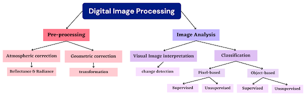
  Prior to the analysis of remote sensing systems, they undergo a pre-processing stage . However, the radiation received by satellite sensors is subject to various phenomena that introduce radiometric and geometric distortions. As a result, two types of correction are required: atmospheric correction and geometric correction. During the atmospheric correction, the light detected by the satellite sensor differs from the light reflected by objects on the Earth's surface. The radiation reaching the sensor, known as reflectance , is influenced by the presence of the atmosphere. In contrast, the unaltered radiation is referred to as radiance . To accurately interpret the characteristics of the Earth's surface, it is necessary to eliminate the atmospheric influence and obtain the true reflectance values. Geometric correction is a crucial step in image acquisition to address distortions that can result in significant disparities between the actual Earth coordinates and the correspo

Remote Sensing System

Image
  Remote sensing systems can be categorized into two types: active and passive. Active remote sensing systems utilize their own source of illumination, emitting pulses of light and measuring the backscatter reflected to the sensor. On the other hand, passive remote sensing systems rely on the measurement of sunlight that is naturally emitted by the sun and reflected from the Earth's surface. When the sun is shining, passive sensors capture and measure this energy for analysis. There are three types of active remote sensing systems: radar, sonar, and lidar. Radar emits out radio waves and then detects the signals that bounce back. Various types of radar images include specular reflection, double-bound, and diffuse scattering. Sonar emits sound waves and measures their echoes in water. Lidar emits beams of light and measures their reflections. Diagram above shows the medium of transmission.  Remote sensing involves the use of radiation, which needs to interact with the atmospher

Project 5: Normalized Difference Vegetation Index (NDVI)

Image
The Normalized Differentiation Vegetation Index (NDVI) is an index introduced in 1979 by Tucker to measure the health and density of vegetation. It compares the reflectance difference between Near Infra-Red (NIR) and Red bands . NDVI is commonly used to assess green biomass, leaf area index, and production patterns. The values of NDVI range from -1 to 1, with low values indicating barren areas, moderate values indicating sparse vegetation, and high values indicating dense vegetation. Table above shows the land cover classification of NDVI value NDVI can be obtained by calculating the ratio using satellite images. It is useful in land cover classification as it can differentiate different types of land cover based on the percentage of red light reflected back into space. The equation above uses the near infra-red values and red values. To obtain Landsat images, the USGS Earth Explorer platform is utilized. A dataset covering the period from October 1, 2022, to March 29, 2023, with a 30%

Project 4: Land Surfuce Temperature Analysis

Image
In the past, weather stations have been used to measure surface temperature, but limited station coverage has led to incomplete datasets. However, land surface temperature (LST) datasets derived from satellite measurements offer high-resolution and wide coverage, especially for studying urban heat island effects. Satellite technology, such as  Moderate Resolution Imaging Spectroradiometer ( MODIS), provides precise temporal and spatial resolution for LST estimation. The LST value can be extracted through pixel-based calculation. The value of each pixel will be calculated by using equation 1 (Wan, 2007):     𝑳𝒂𝒏𝒅 𝒔𝒖𝒓𝒇𝒂𝒄𝒆 𝒕𝒆𝒎𝒑𝒆𝒓𝒂𝒕𝒖𝒓𝒆 (𝒊𝒏 °𝑪) = (𝑝𝑖𝑥𝑒𝑙 𝑣𝑎𝑙𝑢𝑒 × 0.02) − 273.15 To obtain LST values, the study area (Cameron Highlands) is extracted from a shapefile, and monthly LST is derived by compositing four satellite images. The composite image's projection is adjusted to ensure proper alignment with the Earth's surface, as an incorrect coordina

Introducing Remote Sensing

Image
  Remote Sensing is a technique to obtain information about the properties of an object without physically contacting it from a distance. In contrast to field-based measurement, remote sensing offer advantages in terms of time, cost, and also energy efficiency. It allows for the coverage of larger areas and is more effective compared to field-based measurement. Remote sensing involves several steps, including planning the mission and choosing the suitable sensors, receiving and recording the signal data, and the analyzing the resultant data. Satellites used in remote sensing do not directly measure the Earth's geophysical parameters. Instead, satellites will observe, capture and measure solar and terrestrial radiance (light) present in a vertical column of the atmosphere. These radiance measurements are then converted into geophysical parameters through the application of science-based algorithms (physics, assumptions and so on).  There are seven process components of remote sensin

Attribute Data Management

Image
  Attribute data refers to non-spatial information that provides details about a spatial feature. Spatial data includes both location information and additional attributes accompanied with it. There are two methods for linking the tables: joining and relating. Joining a table involves establishing a  temporary relationship between tables through a relational Data Based Management System (DBMS). The tables need to have a common field and the original stored data remains unaffected. Calculation views can apply a cardinality setting to joins which specifies the number of matching entries in the other tables for each entry in one table. Cardinality types include one-to-one, one-to-many, many-to-one and many-to-many. On the other hand, relating tables are similar to joins but the tables remain separate and selected items in one table may be highlighted in the table.  A query is used to extract specific records from a table based on specified conditions. Many databases utilize a specialized

Raster Geoprocessing Toolkit

Image
  In GIS, there are two types of basic geoprocessing with raster data analysis: single layer analysis and multiple layer analysis. For the single layer analysis, reclassification or recoding is basically assigning a new range of values to all pixels in the dataset based on their original values. This simplification allows for fewer unique values and cheaper storage requirements. Buffering for raster data tends to approximations representing those cells that are within the specified distance range of the target. For the multiple layer analysis, the clipping process of raster data results in a single raster that is identical to the input raster but shares the extent of the polygon clip layer. The overlay process of raster data is that the number within the aligned cells of the input grids can undergo any user-specified mathematical transformation. The Boonlean raster overlay methods can use the connector (AND, OR and XOR) to combine the information of two overlying input raster data sets

Project 3: Soil Erosion Analysis

Image
Upon initial observation, Kampung X is currently facing a severe issue with erosion. As a researcher assigned by the Department of Agriculture Malaysia, my responsibility entails 1the task of conducting studies on the soil erosion rate from 1990 to 2010. The Revised Universal Soil Loss Equation (RUSLE) is used as it can estimate erosion and plan conservation measures by predicting the amount of soil loss in specific fields with specific slopes. This equation utilizes five key factors that can be assigned numerical values to predict the soil loss at a given location. The soil loss is calculated as follows: A = R × K × LS × C × P   where A is annual soil loss (tons/ha/yr),  R is the rainfall erosivity factor,  K is the soil erodibility factor,  LS is slope length and steepness factor,  C is cropping and management factor, and  P is conservation supporting practices factor (Yoder and Lown, 1995) Rainfall erosivity (R) factor is the index that measures the erosion force of specific rainfa

Vector Geoprocessing Tools

Image
A geoprocessing tool is one that systematically manipulates either the geometry or the attribute information or both of a vector GIS data file. It is used to perform various spatial operations and analyses on vector data. These tools allow for tasks such as buffering, clipping, merging, intersecting, dissolving, and more. They provide the means to extract, transform, and analyze data within a geographic context, facilitating effective spatial analysis and decision-making processes.   The photo above clearly shows the function of the 6 basic toolkits. Basic six toolkits Buffer - creates a geometric area around vector features by using points, lines or polygons (input) at a specified distance of a feature or features (buffer width) - can create variable distance buffers based on attribute value  - use equidistant projection to center the point from that point, know the scale well and can draw buffer Clip   - subset tool - large dataset to clip down into smaller subset/dataset - clip oper

Project 2: Land use change analysis

Image
    To analysis the land use change by using GIS The land use change map  for the Year 1990 to 2000, 2000 to 2010, and 1990 to 2010 are created using QGIS . The graph of land use changes for the Year 1990 to 2000, 2000 to 2010, and 1990 to 2010 are drawn by using Microsoft Excel .  Diagram above shows the map of land use change from the year 1990 to 2000. Graph above shows the area change (hectare) of land use change from the year 1990 to 2000. Diagram above shows the map of land use change from the year 2000 to 2010. Graph above shows the area change (hectare) of land use change from the year 2000 to 2010. To get a better visual for soil erosion change for the past 20 years, a map and a graph is drawn.  Diagram above shows the map of land use change from the year 1990 to 2010. Graph above shows the area change (hectare) of land use change from the year 1990 to 2010.      From the graphs, the area of forest is the largest and the orchard has the second largest area no matter from the y